6.5 Closed-Form Solutions for Trajectory Parameters
Mayevski’s choiceThis autby those ballisticians, but these solutions are not published in any references available to us. We have found them useful because they are exact solutions to Siacci’s equations of motion and they obviate the necessity of numerical integration techniques and the inaccuracies associated with those techniques.
To see how the closed-form solutions are derived, let us begin by substituting equation (6.4-1) into equations (6.3-13) through (6.3-16). The results are:
 (6.5-1) (6.5-2) (6.5-3) (6.5-4)
Note that in these substitutions
Equations (6.5-1) and (6.5-2) can be integrated directly. Let us integrate the equations between an initial pseudovelocity u 1 and a final pseudovelocity u 2 , both of which are in the same subrange k :
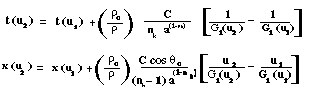 (6.5-5) (6.5-6)
Equation (6.5-6) is correct for all but the final subrange 9 where n 9 = 1 . In that subrange:
Equation (6.5-4) can also be integrated directly. However, to solve equation (6.5-3), we must first integrate (6.5-4) from u 1 to a value u , substitute that result into (6.5-3), and finally integrate the result of those steps. The final results are:

 (6.5-9)
In equations (6.5-8) and (6.5-9) the symbols (tan X) 1 and (tan X) 2 mean the slope of the trajectory evaluated at u1 and u2 , respectively.
Equations (6.5-5) through (6.5-9) are the closed-form solutions for the bullet trajectory (the time of flight, range slope, and vertical position) within any single pseudovelocity subrange denoted by k . When the bullet is fired, it begins flight at a velocity
in one of the subranges. As it flies, it slows down. When the pseudovelocity reaches the boundary of that subrange
we must then calculate the time of flight, range, slope, and vertical position at that boundary value. Then we must change subrange coefficients A k and n k to their new values A k+1 and n k+1 . After that we can continue to compute the trajectory in the new subrange, using the boundary values of the trajectory parameters as initial conditions for the new subrange.