6.2 Drag Force and the Drag Function
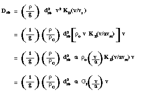
Turning now to a description of the drag force D on a bullet, we first consider the drag on the standard bullet. The firing tests performed around the turn of the century revealed that the aerodynamic drag force on a bullet is a function of the air density through which the bullet flies, the axial cross-sectional area of the bullet upon which the drag acts, the velocity of the bullet, and the speed of sound. The research conducted at that time showed that the drag on the standard bullet can be expressed by the following equation:
In this equation the subscript sb denotes the parameters which are peculiar to the standard bullet. The parameter r m is the mass density (slugs/cu ft) of the air, d is bullet diameter, v is bullet velocity, vs is the speed of sound, and K D is a function of the bullet Mach number v/v s . K D also includes the constant X/4 which, when multiplied by d 2 expresses the bullet cross-sectional area.
The mass density r m of air is not a readily available parameter, but the weight density r (lbs/cu ft) is listed in almost every reference on atmospheric conditions. The two densities are related by:
Now, consider the drag on the standard bullet at sea level standard atmospheric conditions:
Where r o is the standard weight density of air and V so is the standard speed of sound at sea level.
Rearranging the terms:
The term in the square brackets in equation (6.2-4) is defined to be the drag function G 1 :
G 1 (v) is a function only of bullet velocity v because r o and v so are constants. Substituting equation (6.2-5) into (6.2-4) yields:
At any altitude other than sea level both the air density and the speed of sound change. For standard (dry air) atmospheric conditions at any altitude, the equations that we recommend for calculating air density and speed of sound are:
r = r o exp(-3.02149 x 10 -5 (L + y)) (6.2-7)
v s = a v so (6.2-8)
a – 1.0 – 1.126666 x 10 -5 (L + y) – 6.753074 x 10 -11 (L + y) 2 (6.2-9)
Where L is the altitude of the firing point and y is the vertical coordinate of bullet position (seeFigure 6-1 ). For small arms trajectories, the vertical coordinate effects on r and a negligible, and (L + y ) is replaced by ( L ) in equations (6.2-7) and (6.2-9).
Now, let us write the drag on the standard bullet at any altitude:
 (6.2-10)
Equation (6.2-10) shows explicitly that at any altitude other than sea level there are two distinct effects on drag. First, there is a correction for the air density change, which is the factor r / r o in equation (6.2-10). Second there is a correction for the speed of sound change which is the factor [ a G 1 (v/a) ] in the equation.
Next, we turn to the question of how to express the drag on a bullet other than the standard bullet. We can imagine repeating the drag determination tests on the new bullet, and we would expect a result similar to equation (6.2-10), with d sb replaced by the diameter of the new bullet and a different factor replacing K D . But if we had to repeat such a test sequence for every bullet, it would be tedious and enormously costly.
Instead, ballisticians around the turn of the century made an assumption of great importance to small arms ballisitics. This assumption is that the drag function G(v) for a bullet which is generally of the same shape as the standard bullet is related to G 1 (v) simply by a constant scale factor. In other words, the drag force on such a bullet can be expressed by the equation:
where d is the bullet diameter and i is the scale factor, known as the form factor. All other parameters are as defined above. Equation (6.2-11) then expresses the drag on any bullet of the same general shape as the standard bullet for atmospheric conditions at any altitude. If equations (6.2-7) and (6.2-9) are used to calculate r / r o and a , then (6.2-11) expresses drag force for standard atmospheric conditions at the altitude of the firing point.
The final step in this section is to substitute equation (6.2-11) into equations (6.1-2) and (6.1-3). After dividing through by m and substituting (6.1-5), we obtain:
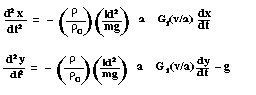 (6.2-12) (6.2-13)
In these equations we can immediately recognize the bullet ballistic coefficient:
where w is the bullet weight in pounds and bullet diameter d is in inches. The standard bullet for G1 (v) has a weight of one pound, a diameter of 1 inch, and form factor defined to be unity. Therefore, the ballistic coefficient of the standard bullet is
Rewriting equations (6.2-12) and (6.2-13) using the ballistic coefficient yields:
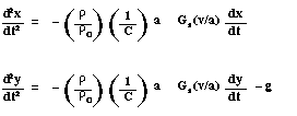 (6.2-15) (6.2-16)
These are the differential equations of motion of the bullet. They are nonlinear and coupled because
To solve these equations directly requires numerical integration. However, Siacci and Mayevski made contributions which simplified these equations further.